import pandas as pd
import numpy as np
from math import *
import matplotlib.pyplot as plt
Processing time for array creation.
Let's explore different ways of creating an N=1000 element array:
Below are some append() operations we've done many times to list and numpy arrays.
We can determine their runtime using the %%timeit magic variable in Jupyter. %%timeit runs multiple experiments or 'loops' to estimate the mean and standard deviation in the processing time.
%%timeit -n 100
# Appending items to a list array.
N = []
for n in range(1000):
    N.append(n)
Append() operation on numpy arrays...
%%timeit -n 100
# Appending items to a Numpy array
N = np.array([]);
for n in range(1000):
    N = np.append(N,n)
Finally, create the array as Numpy would recommend to do it.
%%timeit -n 100
N = np.arange(0,1000,1)
Results: Clearly, np.arange() is not using a for-loop, at least not in Python language, because this operation is much faster than even the base-python list array loop.
How does the time required for computation scale with the value of N?
- Instead of using
%%timeit, use the time() module to calculate the compute time. - Do this for multiple values of N.
- Normalize or divide the compute time by the first value, so the compute time is unitless. This lets us compare with the benchmark curves below.
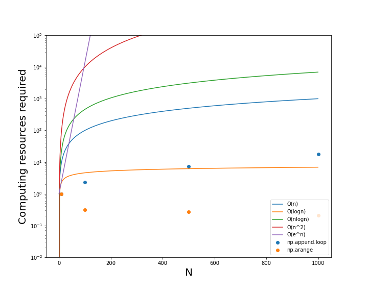
The goal will be to reproduce this figure for different operations in Numpy and Pandas.


## Code to test how compute time scales with N, the number of computations.
## Annotate this code together in class.
import time

# Create ....
Ns = [10,100,500,1000]

## LOOP1:
t = []
for i in Ns:
    ti = time.time()
    N = np.empty([0,i]);
    for n in range(i):
        N = np.append(N,n)
    t.append(time.time()-ti)

t = np.array(t)/t[0]
print(t)

## LOOP2:
t2 = []
for i in Ns:
    ti = time.time()
    N = np.arange(0,i,1)
    t2.append(time.time()-ti)

t2 = np.array(t2)/t2[0]
print(t2)
Algorithm efficiency benchmarks developed by Don Knuth.
- Make graphs of the Benchmark scaling relationships between N and the compute time.
- Compare these curves to the append() results.
N = np.arange(0,1e3,1)    # Create an O(n) vector for graphing.
N = np.array(N,ndmin=2).T
Ologn = np.log(N);         # Create an O(log(n))  vector for graphing.
Onlogn = N*np.log(N);      # Create an O(n*log(n)) vector for graphing.
On2 = N**2;                # Create an O(n*n) vector for graphing.
Oexp = 1.1**N              # Create an O(e^n) vector for graphing.
AN = np.concatenate((N,Ologn,Onlogn,On2,Oexp),axis=1)

plt.figure(figsize=(10,8))
plt.plot(N,AN);
plt.ylim(1e-2,1e5);
plt.yscale('log')
#plt.xscale('log')

plt.scatter(Ns,t,s=50,marker='s')
plt.scatter(Ns,t2)
plt.legend(['O(n)','O(logn)','O(nlogn)','O(n^2)','O(e^n)','np.append.loop','np.arange'])

plt.xlabel('N',fontsize=20)
plt.ylabel('Compute time required',fontsize=20)

#plt.savefig('Compute_resources.png')
Results: The np.append() loop scales somewhere between O(log(n)) and O(n) suggesting it is relatively efficient, even though it is much slower than np.arange(), which actually decreases in compute time for larger values of N. This suggests that np.arange() is actually O(1) or has a constant compute time.
NOTE: The rest of this tutorial is copied directly from Sofia Heisler's excellent Pycon presentation on optimizing Pandas code.
What does efficient code in Pandas and Numpy look like?
# Load in the data file for computation
df = pd.read_csv('new_york_hotels.csv', encoding='cp1252')
df.head()
Haversine definition
Haversine function computes the great circle distance between two lat/lon locations on the globe.
def haversine(lat1, lon1, lat2, lon2):
    miles_constant = 3959
    lat1, lon1, lat2, lon2 = map(np.deg2rad, [lat1, lon1, lat2, lon2])
    dlat = lat2 - lat1
    dlon = lon2 - lon1
    a = np.sin(dlat/2)**2 + np.cos(lat1) * np.cos(lat2) * np.sin(dlon/2)**2
    c = 2 * np.arcsin(np.sqrt(a))
    mi = miles_constant * c
    return mi
1. Crudest looping
Using the for loop to iteratively access row-wise elements in the Pandas Dataframe does not take advantage of the vectorized capabilities that Pandas can achieve (through Numpy).
# Define a function to manually loop over all rows and return a series of distances
def haversine_looping(df):
    distance_list = []
    for i in range(0, len(df)):
        d = haversine(40.671, -73.985, df.iloc[i]['latitude'], df.iloc[i]['longitude'])
        distance_list.append(d)
    return distance_list
%%timeit
# Run the haversine looping function
df['distance'] = haversine_looping(df)
2. Iterrows Haversine
Pandas offers an row-wise iterator that is faster than indexing via a loop.
%%timeit
# Haversine applied on rows via iteration
haversine_series = []
for index, row in df.iterrows():
    haversine_series.append(haversine(40.671, -73.985,\
                                      row['latitude'], row['longitude']))
df['distance'] = haversine_series
3. Apply() Haversine on rows
%timeit df['distance'] =\
df.apply(lambda row: haversine(40.671, -73.985,\
                               row['latitude'], row['longitude']), axis=1)
4. Vectorized implementation of Haversine applied on Pandas series
# Vectorized implementation of Haversine applied on Pandas series
%timeit df['distance'] = haversine(40.671, -73.985,\
                                   df['latitude'], df['longitude'])
5. Compute Haversine on rows in Numpy instead of Pandas
DF = df.iloc[:,[6,7]].values  # Convert Pandas columns into a Numpy array

%timeit [haversine(40.671, -73.985,row[0], row[1]) for row in DF]
6. Vectorized implementation of Haversine applied on NumPy arrays
np_lat = df['latitude'].values
np_lon = df['longitude'].values

# Vectorized implementation of Haversine applied on NumPy arrays
# %timeit df['distance'] = haversine(40.671, -73.985,\
#                         df['latitude'].values, df['longitude'].values)


%timeit df['distance'] = haversine(40.671, -73.985,\
                         np_lat, np_lon)
Cythonize that loop
Future: The fastest python code uses precompiled C code, which is available through the Cython module.
7. In-class assignment: Benchmark and graph haversine methods 1, 3 and 6.
- Evaluate the haversine functions using N = 10, 100, 500, and 1000 as in the example above with lat/lon pairs of hotels in the world. Hint: subindex df to pass only N values, instead of the full array (which is 1600).
- Use the
ti = time.time(); t = time.time()-ti;code to capture the compute time for graphing. - Normalize t as above.
- Recreate the graph above showing the curves for algorithm performance.
- Graph the output as a function of N's, as above.
8. What to turn in?
- .Png or .jpg image of the benchmark graph with your results from haversine methods 1, 3, and 6 included.