Intro to Dataframes
Dataframes in R provide a sophisticated data structure for organization and analysis including with time series operations.
Check out: https://www.youtube.com/watch?v=edifwfMEL_I
 (c)dataquest.io
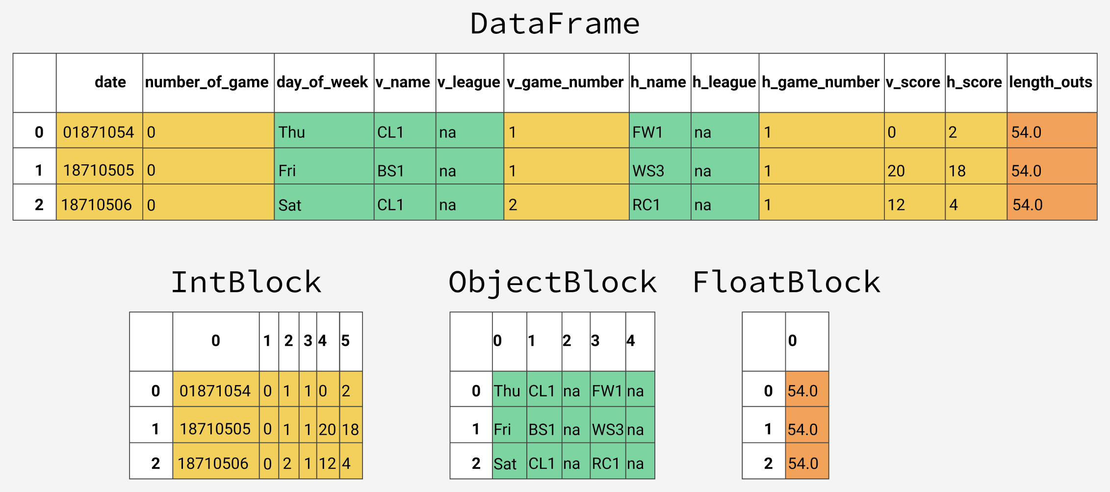
The DataFrame allows us to load a complicated file into Python and perform multiple data manipulations efficiently, and without having to recast the data.
In [ ]:
library(readxl) # Read in Excel files
library(tidyverse)
library(lubridate) # Create and manipulate date objects and time objects.
library(xts) # adds ability to merge data frames on date.
library(dplyr)
library(zoo) # time series features for data frames.
library(patchwork) #
In [ ]:
# Read the Excel file into an R data frame
freight <- read_excel("ScienceInventory_Ioffe.xlsx")
In [ ]:
head(freight, n = 10) # Displays the first 10 rows
In [ ]:
tail(freight, n = 10) # Displays the last 10 rows
In [ ]:
# Summary gives some insight into the data type of each column.  Also note it is shown in the header when you
# type tail or head
summary(freight)
In [ ]:
as.matrix(freight) # You can extract a generic array
In [ ]:
# Read in a text file that is delimited by whitespace.  '\s+' allows multiple whitespace characters to exist
# between each entry.

# If file has a header, you need to tell read_csv() how many rows to skip, or it will misinterpret the shape of the
# dataframe.

ts = read.csv('20151028 blank test.asc',sep='\t',skip=7)
head(ts,n=10)
In [ ]:
# This is timeseries data, so we should utilize a datetime data type as the row index.
# First, we have to create datetime.

fname = 'timeseries2.txt'
# Read in the data and specify all columns as character arrays.  Otherwise we lose leading zeros in the time column.
ts = read.csv(fname,sep=',',skip=1,header=FALSE,colClasses="character")
# Add the strings together, convert them to a datetime and save the result in column 3.
head(ts,n=10)

# specifying the format
format <- "%Y%m%d %H%M"

# combining date and time into single object and put it into a new column in the data frame.
ts$datetime = as.POSIXct(paste(ts$V5, ts$V6), format=format)
Trim bad or unwanted data
In [ ]:
# Use boolean arrays to shorten a dataframe before a time interval.

# Create a begin and end datetime object.
fin <- as.POSIXct('2020-01-03 23:55:00',format='%Y-%m-%d %H:%M:%S')
beg <- as.POSIXct('2020-01-01 10:55:00',format='%Y-%m-%d %H:%M:%S')
#beg <- as.POSIXct('2024-10-22 00:00:00',format='%Y-%m-%d %H:%M:%S')

# Compare the datetime data in ts and get rid of all the data outside of the limits set by beg and fin.
f_ts <- ts %>% filter(ts$datetime >= beg & ts$datetime <= fin)
Fill in missing data.
In [ ]:
# Use na.locf() which stands for "last observation carried forward" to fill in the missing data.

# NOTE xts() can coerce your data into characters if there are non-numeric values in the series.
xts_data <- xts(ts, order.by = ts$datetime)

hr_data <- na.locf(xts_data)
Resample the dataset
In [ ]:
# apply.daily, apply.monthly, apply.weekly, apply.quarterly
hr_day <- apply.daily(hr_data,last)
head(hr_day,n=10)
In [ ]: