Intro to Pandas¶

Pandas is a Python library that provides a sophisticated data structure for organization and analysis. It excels at categorizing data and at time series operations.

Check out: https://pandas.pydata.org/pandas-docs/stable/10min.html https://www.youtube.com/watch?v=F6kmIpWWEdU

Advantages of Pandas

Can read many files: .xls, .csv, any delimited text file, as well as JSON and SQL.
Very smart with identifying data types, e.g. text, integer, float, or even dates.
Allows data indexing along row, column or subrow or subcolumn.
Contains many built-in analysis functions for operating on DataFrames and Series.
Handles missing or empty data.

Dataframes use the dict data type.¶

dict is a way to structure data that allow one to organize the data with names (text).

In [ ]:

# Python example of a dict array.  Note the {} curly brackets and the use of colons.
typo = {'spelling':[2,3,4],'counting':['a','b','c']}

In [ ]:

# Using the label 'spelling' I can access the data regardless of the 
typo['counting'] # indexing in the same way as list[1:10]

In [ ]:

# Dict arrays are easy to Index:
typo['spelling'][1:]

In [ ]:

typo['spelling'].append([5,6])

In [ ]:

# You can even replace values with this easy indexing.
typo['spelling'][1:] = [114,45,66,77]

In [ ]:

typo

NOTE:: Indexing is not quite as easy in Pandas, but still pretty easy.

No description has been provided for this image

(c)dataquest.io

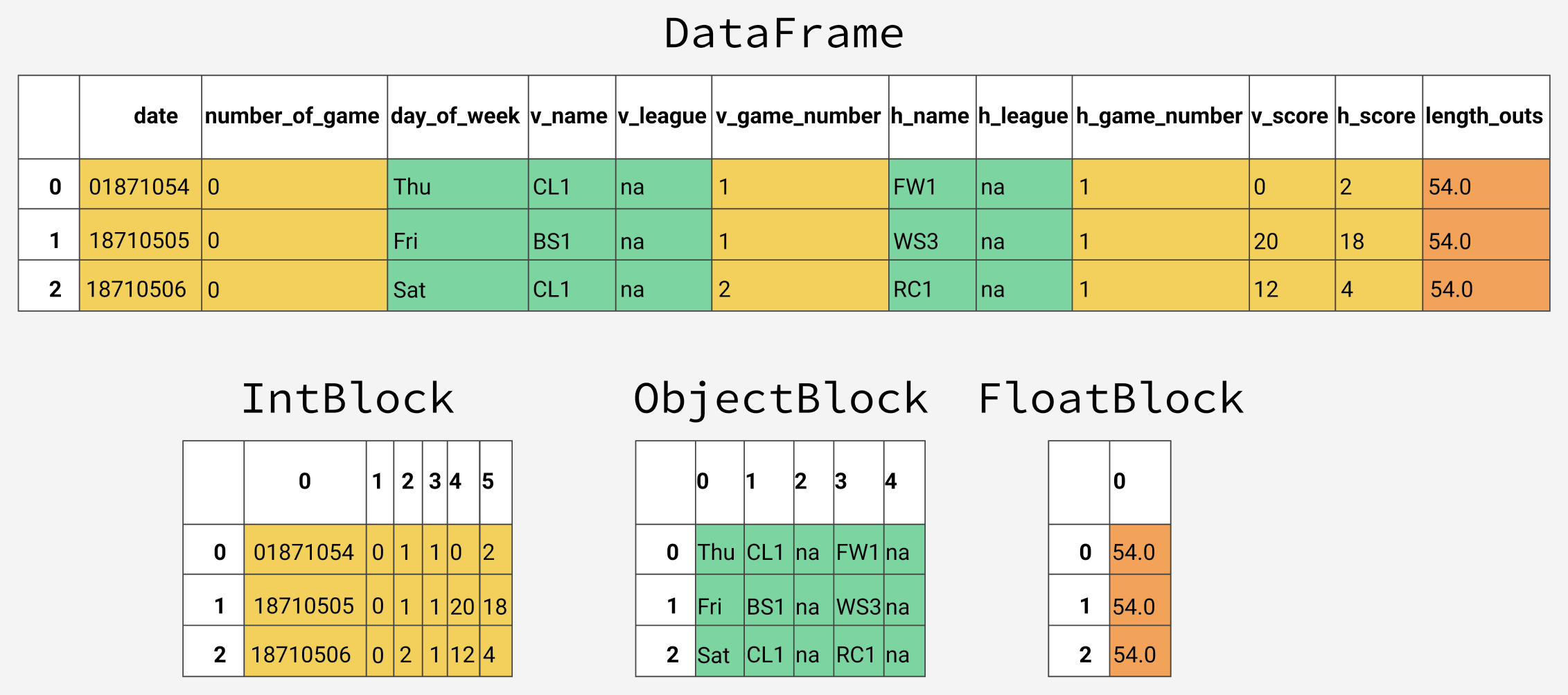
The Pandas DataFrame allows us to load a complicated file into Python and perform multiple data manipulations efficiently, and without having to recast the data.

pd.Series() is analogous to a 1D array, pd.DataFrame() is analogous to a 2D array.
By using indexes to help categorize data and provide a hierarchy of categories. Index applies to row categories.
The column categories are just columns.

In [ ]:

import pandas as pd

In [ ]:

# might be missing openpyxl
# open a terminal and run >> pip install openpyxl
freight = pd.read_excel('ScienceInventory_Ioffe.xlsx')  # might be missing openpyxl
#freight = pd.read_excel('ScienceInventory_Ioffe.xlsx',index_col='Institution')

In [ ]:

freight.head()  # Plot the first five rows of the dataframe

In [ ]:

# Pandas automatically fills in empty data with NaNs.
freight.tail() # Plot the last five rows of the dataframe

In [ ]:

# Pandas is fairly clever about determining the right data type for each column.  
# If it can't determine, the default is text and the dtype is "object".
freight.info()

In [ ]:

# You can extract a generic array from the Pandas dataframe, using the .values attribute.
Array = freight['Weight (lbs)'].values  
Array?

In [ ]:

# Keys are the index terms for each column.
# freight.keys()
freight.columns # The columns object gives the same thing.

In [ ]:

# Change the row index to the 'Institution', instead of the numeric row number.  
# This provides another level of organization and data access, a little bit like an SQL relational database.
freight = freight.set_index('Institution')
freight.head()

In [ ]:

freight['Weight (lbs)']['U. Illinois Chicago']  # Report the weights column for UIC freight.

In [ ]:

freight['Weight (lbs)']['U. Illinois Chicago'].sum()  # Do arithmetic on on the UIC freight.

In [ ]:

# This will fail. Note the reversal of indices.

freight['U. Illinois Chicago']['Weight (lbs)'].sum()  # Pandas specifies column indices first, then row indices.

In [ ]:

# Read in a text file that is delimited by whitespace.  '\s+' allows multiple whitespace characters to exist 
# between each entry.

# If file has a header, you need to tell read_csv() how many rows to skip, or it will misinterpret the shape of the
# dataframe.
ts = pd.read_csv('20151028 blank test.asc',sep='\t',skiprows=7,parse_dates=[0,3])
print(ts.info())
ts.head()

In [ ]:

# This is timeseries data, so we should utilize a datetime data type as the row index.   
# First, we have to create datetime. 

fname = 'timeseries2.txt'
# Read in the data and specify columns 3 and 4 - date and time as string data type.
ts = pd.read_csv(fname,sep=',',skiprows=1,header=None,dtype={4:'str',5:'str'})
# Add the strings together, convert them to a datetime and save the result in column 3.
ts[4] = pd.to_datetime(ts[4]+' '+ts[5])
ts.info()

In [ ]:

# Set the index to be the datetime column.
ts.set_index(ts[4],inplace=True)
ts.head()

In [ ]:

# Pandas provides capabilities to manipulate the time base in your timeseries dataframe.  These are possible, once
# you specify a datetime or time column as the row index, as we did above.

# Upsample, but don't replace the values by any interpolation method.
#ts.resample('1min').asfreq()

# Upsample, but replace the values by the constant forward fill method.
#ts.resample('1min').pad()

# Upsample, but replace the values by a linear interpolation.
# ts.resample('1min').interpolate()

In [ ]:

typo = {'spelling':[2,3,4],'counting':['a','b','c']}

1. Use Pandas to import and preprocess your temperature data.¶

In [ ]:

# 1. Use pandas to up or downsample your temperature data to a 5-min time interval.

2. Use Pandas to import and preprocess nearby weather station data.¶

In [ ]:

# Download 5-min temperature data, for a nearby weather station. Look for the neareest 
# 5-min weather stations in RI. These archives are available at:
# https://www1.ncdc.noaa.gov/pub/data/uscrn/products/subhourly01/2025/
#
# 2. Use Pandas to import the data. The NOAA file will take some special processing to 
# create a datetime array.  Make a timeseries of the weather station temperature and save 
# the plot.

3. What is the time interval that you used for your temperature measurements?¶

In [ ]:

# Use Pandas to up or downsample the timeseries so that it matches a 5 minute sampling 
# interval, just like the weather station data.

4. Subset the weather station data.¶

In [ ]:

# Use boolean operators and the datetime index to make a subset array of the weather station
# data that matches the start and end times your temperature measurements.  
# Another way to do this is to explore using the Pandas merge() function.  NOTE: Read the help
# and try not to ask the bots to do it.