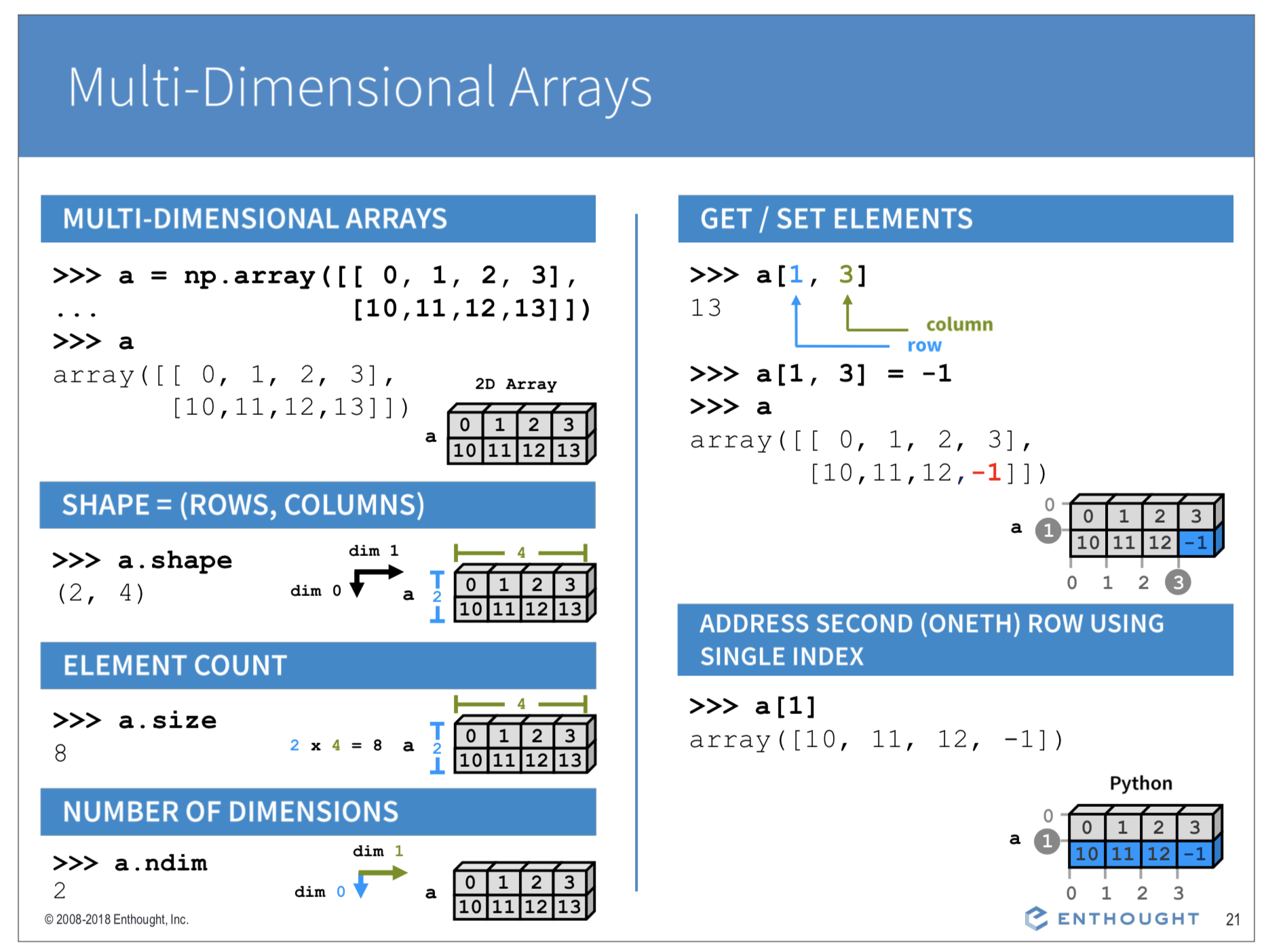
The Enthought PDF slides give further detail on the different types of indexing that exist.
In [ ]:
# PYTHON
# Import modules
import numpy as np
import matplotlib.pyplot as plt
In [2]:
# R. We only need base R for this, because the matrix library is part of base R.
# Import modules
Creating 1D arrays with array() arange() and linspace()
In [ ]:
# Python
# Use array() to create arrays of any dimension if you already know or have the values to put
# into the array.
x = np.array([5,4,3,2,1])

# Linspace inputs are start, stop, # of elements
xls = np.linspace(0,100,100)

# arange inputs are start,stop,interval
xar = np.arange(0,100,0.9999)

#print(xar.shape)
#xls.shape

# This term tells you to pull the last value of the array out
#print( xar[-1], xls[-1])
In [ ]:
# R
# Use array() to create arrays of any dimension if you already know or have the values to put
# into the array.
x <- c(5, 4, 3, 2, 1)

# seq inputs are from, to, and length.out
xls <- seq(0,100,100)
xls <- seq(from = 0, to = 100, length.out = 100)


# arange inputs are start,stop,interval
xar <- seq(from = 0, to = 100, by = 0.9999)

#print(xar.shape)
dim(xar)

# This term tells you to pull the last value of the array out
#print( xar[-1], xls[-1])
Numpy can store numeric information (usually float() or int() data types) in 2, 3 or even N- dimensional arrays. Note that the indexing of 2D arrays goes like [row #, col #], e.g. a[3,2] gives the element at row=4 and column=3.

Creating 2D arrays with array(), zeros(), ones()
In [ ]:
# PYTHON
# Assembling a 2D array by concatenating 1D arrays.
x = np.array([[1,2,3],[3,4,5]])
print(x.shape)

# Currently this is a 1D array
y = np.array([1,2,3])

# Sometimes you need to set an array up to be 2D, so you can add data to it later.
# This should be a 2D array
y2 = np.array([1,2,3],ndmin = 2)

#print("Y has",y.ndim,"dimensions. Y2 has",y2.ndim,"dimensions")
In [ ]:
# R
# Assembling a 2D array by concatenating 1D arrays.
x <- matrix(c(1, 2, 3, 3, 4, 5), nrow = 2, byrow = TRUE)
print(dim(x))

# Currently this is a 1D array
y <- c(1, 2, 3)

# Sometimes you need to set an array up to be 2D, so you can add data to it later.
# This should be a 2D array
y2 <- matrix(c(1, 2, 3), nrow = 1)

# Print the dimensions
print(paste("Y has", length(dim(y)), "dimensions. Y2 has", length(dim(y2)), "dimensions"))
In [ ]:
y*y2
Arithmetic on Arrays (element-wise or linear algebra)
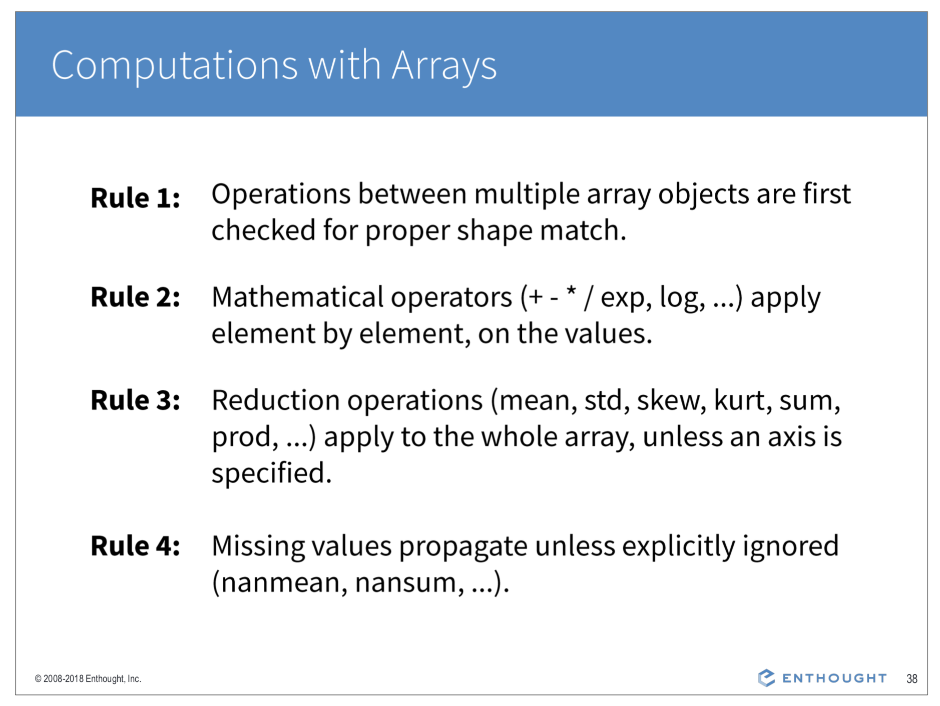
By default, Numpy will try to carry out element-wise arithmetic (+,-,*,/) on arrays of like dimension. Where possible, Numpy will also use array broadcasting to make the operation work.

In [ ]:
# PYHON AND R
y + y2  #This is permitted.  It takes on the higher dimensions.
y * y2  #Likewise permitted.  It takes on the higher dimensions.
In [ ]:
# PYTHON
# Examples of array manipulations.

R = np.arange(0,100,12)  # Create a vector of 9 elements

# Element-wise operation.  P is the same size as R.
P = R*R

# Impliclit element-wise operation.

Q = P.copy() - 3
Q = P*R

# Make R into a 3 x 3 matrix (2D array), and store it in S.
S = R.reshape(3,3)

# An array multiplication with broadcast operation.
T = S*np.array([3,2,1])
#print(T)
In [ ]:
# R
# Examples of array manipulations.
R <- seq(from = 0, to = 100, by = 12)  # Create a vector of 9 elements

# Element-wise operation.  P is the same size as R.
P <- R * R

# Implicit element-wise operation.
Q <- P - 3
Q <- P * R

# Make R into a 3 x 3 matrix (2D array), and store it in S.
S <- matrix(R, nrow = 3, byrow = TRUE)

# An array multiplication with broadcast operation.
T <- S * c(3, 2, 1)
print(T)
In [ ]:
# PYTHON
# (Object-oriented notation, Functional notation)
print(T.max(axis=0),np.max(T,axis=0) )  #Take the max along the row axis
In [ ]:
# R
# Object-oriented notation
print(apply(T, 1, max), max(T, along = 1))  # Take the max along the row axis
In [ ]:
help(apply)
Combining arrays for data wrangling.
In [ ]:
#In general, when concatenating (merging or pasting together) arrays they must have the same shape and same dimensions

#help(np.concatenate)
np.concatenate((y,y2))  # Not permitted.

np.concatenate((y[np.newaxis,:],y2))   #Expand the dimensions of y before concatenating.

# Stack vertically.  This has same effect as concatenate
np.vstack((y,y2))   # Permitted, because arrays have the same column dimensions


# Stack horizontally.
np.hstack((y[np.newaxis,:],y2))   # Not Permitted, because y and y2 have the different row dimensions

#np.hstack((y[np.newaxis,:],y2))
In [ ]:
# R
# In general, when concatenating (merging or pasting together) arrays they must have the same shape and same dimensions
## GEMINI NOTES:
# In R, the equivalents for concatenating arrays along different axes are:
#
#    c(): Concatenates elements along the first dimension (rows).
#    rbind(): Concatenates matrices or data frames row-wise.
#    cbind(): Concatenates matrices or data frames column-wise.
#
# The rbind() function is used to expand the dimensions of a vector before concatenating it with a matrix,
# similar to the np.newaxis operation in Python.

# help(np.concatenate)
c(y, y2)  # Not permitted.

rbind(y, y2)  # Expand the dimensions of y before concatenating.

# Stack vertically.  This has same effect as concatenate
rbind(y, y2)  # Permitted, because arrays have the same column dimensions

# Stack horizontally.
cbind(y, y2)  # Not Permitted, because y and y2 have the different row dimensions
Indexing and boolean operations for 2D arrays
In [ ]:
# PYTHON

z = np.ones((100,50)) # Make a 2D array of ones that is 100 x 50.

# Index individual row or column in 2D array

# Save a single row of z to a new variable
zr = z[9,:]

# Save a single column of z to a new variable
zc = z[:,9]

print(zc.shape,zr.shape, z.shape)
In [ ]:
# R

z <- matrix(1, nrow = 100, ncol = 50) # Make a 2D array of ones that is 100 x 50.

# Index individual row or column in 2D array

# Save a single row of z to a new variable
zr <- z[9, ]

# Save a single column of z to a new variable
zc <- z[, 9]

print(dim(zc), dim(zr), dim(z))
In [ ]:
#print(z)
In [ ]:
# Make a 2D column vector with 10 elements in it.
a = 3.2*np.ones([10,1])

# Copy that column vector 10 times to make a square array.
b = np.tile(a,10)


# Make a vector of 10 elements and then place them in the diagonal of a 10 x 10 square array.
c = np.ones(10)*100
d = np.diag(c)

# Use the Matplotlib spy() function to visualize the array b+d
plt.spy(b+d,precision=10,markersize=10)
plt.show()

#print(b+d)


#np.random.randn(10)
In [ ]:
# Make a 2D column vector with 10 elements in it.
a <- 3.2 * matrix(1, nrow = 10, ncol = 1)

# Make a 10 x 10 array.
b <- 3.2 * matrix(3.2, nrow = 10, ncol = 10)


# Make a vector of 10 elements and then place them in the diagonal of a 10 x 10 square array.
c <- 100 * rep(1, 10)
d <- diag(c)

# Use equivalent R functions to visualize the array b + d
library(ggplot2)  # Load ggplot2 for visualization

# Create a data frame for ggplot
data <- data.frame(x = seq(1, 10), y = seq(1, 10), z = b + d)

# Create the plot (I was not able to find the equivalent solution in R).
# ggplot(data, aes(x = x, y = y, fill = z)) +
#  geom_raster() +
#  scale_fill_gradient(name = "Values", low = min(b + d), high = max(b + d)) +
#  coord_fixed() +
#  labs(title = "b + d", x = "X-axis", y = "Y-axis") +
#  theme_void()

# No need for plt.show() in R, the plot is displayed automatically
In [ ]:
#help(t)
In [ ]:
# PYTHON AND R
# Check out shape, ndim, dtype
z = d+b

#print(z.shape)

#print(z.dtype)

#print(z)
In [ ]:
# PYTHON
# Use boolean operators to change values.

z2 = z.copy()

# Find all the values equa1 to 1.
id1 = (z2 == 1)

# id1 now has a boolean record of which values are ==1.
print(id1)
In [ ]:
# R
# Use boolean operators to change values.

z2 = z

# Find all the values equa1 to 1.
id1 <- z2 == 1

# id1 now has a boolean record of which values are ==1.
print(id1)
print(z2)
In [ ]:
# PYTHON AND R
# Let's change all the elements equal to 1.

z2[id1] = 3.14159

#z2[z2 == 3.14159] = np.nan

print(z2)
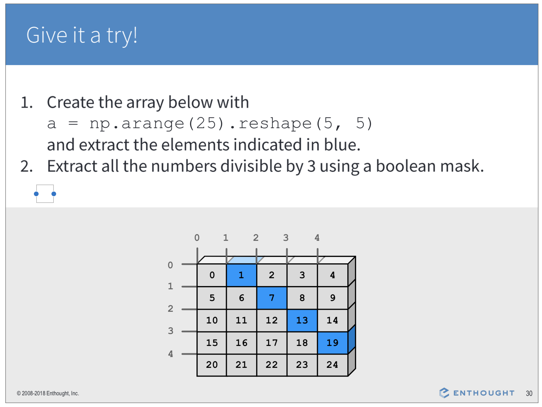
Let's try this exercise together. How many ways can this be solved, algorithmically?

Algorithm 1:
- Create a
- Divide all elements by 3.
- Look for values with a remainder of zero.
- Create boolean array to subindex.
Algorithm 2:
- Create a
- Divide all elements in a by 3.
- Check to see which elements are equal to their integer counterparts.
Finish the notebook by solving the cells below with code.
In [ ]:
# Convert all the values of z2 that are > 99 into NaNs.
In [ ]:
In [ ]:
# Make a 2D numpy array named Arr of size 10 x 10 and fill it with random values that range between 0 and 99. You can use numpy's random module
In [ ]:
# Use boolean indexing to replace all the values in Arr greater than 80 and less than 20 with NaNs.
In [ ]:
# Use the append() or concatenate() commands in numpy to add more columns to Arr.
Concept Review: More looping practice
In [ ]:
# We already saw that np.diag() can insert elements along the diagonal of a square array.
# Use your understanding of for loops to carry out the same operation.
# Create a 10 x 10 array of ones and then modify the center diagonal to be 101 instead of 1.
# Hint: You will need two indices, e.g i and j to specify the row and column to modify.
# Hint: You can use a boolean operator to decide which elements in the square array to modify.